Repository navigation
Conversation



The cold-plasma Hamiltonian becomes H = N_perp^2 - n_perp^2(N_par^2, X, Y), where
n_perp^2 is the O- or X-mode root of the dispersion relation written as a quadratic
in N_perp^2 at fixed N_par (dispersion.refractive_index_perp_squared_cold). The
Appleton-Hartree form in the angle to B has a conical point at X = 1, theta = 0,
which is the image of the whole O-mode cutoff segment {X = 1, N_perp = 0,
N_par^2 < Y/(1+Y)}: every oblique O-mode reflection passes exactly through it, the
gradient of H has no limit there, and the ray can continue on the X-mode sheet. The
fixed-N_par root has no branch point for X <= 1, its discriminant factorises as
X^2 Y^2 [Y^2 (1 - N_par^2)^2 + 4 N_par^2 (1 - X)] (no cancellation at low density),
the + root is the O mode for every Y, and it depends on N_par only through N_par^2,
so N_par = 0 needs no guard.

Rays are integrated in Hamiltonian time, dr/dt = dH/dN, dN/dt = -dH/dr, instead of
the arc length: at the cutoff the group velocity vanishes (P = 0 gives the
determinant a factor N_perp^2), the path has a cusp and the arc-length right-hand
side is 0/0 there, whereas in Hamiltonian time the reflection is a regular point.
The arc length rides along as the eighth state component, ds/dt = |dH/dN|: it stays
the coordinate of the output profiles and of max_arc_length, but it is left out of
the error norm of the PID controller, so the step sequence is that of the state
without it. Its increment over a step serves the controller to apply max_step_size
in metres and to reject steps longer than 1.5 max_step_size.

The step error adds the frequency mismatch delta omega / omega = Delta H /
(omega dH/domega|_k), with omega dH/domega|_k = omega dH/domega|_N - N . dH/dN, to
the PID error instead of Delta H / (2|N|). It has the same meaning for any form of H
and stays finite at the reflection.

The public API is unchanged. max_arc_length becomes a second termination condition
on the arc length, root-found like the exit from the plasma, so the ray ends at that
length itself and TraceResult.incomplete is set as before. The termination event
keeps rho > 1.05, exp(-tau) < 1e-3 and |r| > 20 m.

The theory page of the docs describes the fixed-N_par root, the Hamiltonian-time
integration and the frequency mismatch, with the two root maps as a figure; the
limitations page lists the OX conversion and gap, the fold of the root beyond the
cutoff for the X mode at Y > 1 and the missing stop at the upper-hybrid resonance;
the tuning page says what dispersion_error_weight measures. The sign of the O mode
in the Appleton-Hartree formula on the theory page is corrected.

Benchmarks (analytic tokamak, O and X mode below, above and across Y = 1): all
O-mode reflections of the mode scan end within 1 mm of the converged run with the
shipped settings; the OX reflection scan reflects 10 of 10 launches (PR proximafusion#89: 2 of
10), and d(end point)/d(launch angle) through a reflection agrees with central
differences to 0.3 %. Known limits: a sub-wavelength evanescent OX gap can be
crossed depending on the step placement, the fixed-sign root folds for the X mode
at Y > 1 beyond X = 1 + Y^2 (1 - N_par^2)^2 / (4 N_par^2), and there is no stop
event at the upper-hybrid resonance.


Collaborator
|
I ran the Travis validation scans (based on W7-X) on this branch stacked on top of #90 and I can confirm
Of course this validation scans doesn't test the reflections, so it's only useful as a cross-check showing that there is no regression. I did find one regression though: In the step 1 scan (no absorption, only trajectory), 61 of the rays reach |

DavidMStraub
added a commit
that referenced
this pull request
Nov 13, 2026
The dispersion term of the step-size controller now divides the change of H
by |ω ∂H/∂ω| at fixed wave vector, i.e. it controls the relative frequency
mismatch δω/ω instead of |ΔH|/(2|N|). The measure does not depend on how H
is normalized and equals the change of |N| in vacuum, as before.

Taken from #91 by @alpxp.
This branch has not been deployed
This file contains hidden or bidirectional Unicode text that may be interpreted or compiled differently than what appears below. To review, open the file in an editor that reveals hidden Unicode characters.
Learn more about bidirectional Unicode characters
Sign up for free
to join this conversation on GitHub.
Already have an account?
Sign in to comment


Add this suggestion to a batch that can be applied as a single commit.This suggestion is invalid because no changes were made to the code.Suggestions cannot be applied while the pull request is closed.Suggestions cannot be applied while viewing a subset of changes.Only one suggestion per line can be applied in a batch.Add this suggestion to a batch that can be applied as a single commit.Applying suggestions on deleted lines is not supported.You must change the existing code in this line in order to create a valid suggestion.Outdated suggestions cannot be applied.This suggestion has been applied or marked resolved.Suggestions cannot be applied from pending reviews.Suggestions cannot be applied on multi-line comments.Suggestions cannot be applied while the pull request is queued to merge.Suggestion cannot be applied right now. Please check back later.
Trace in Hamiltonian time with the N⊥² root at the ray's N∥
Follow-up to #89. A ray reflected at its cutoff is the most ordinary event in an ECRH ray tracer, and$H$ , and changes three things: what $H$ is, what the independent variable is, and what the step error measures. The same rays then reflect where they should, with the shipped settings within a millimetre of the converged run, and the solve is differentiable through the reflection. The public API is unchanged.
mainafter #89 still gets it wrong: with the shipped settings a reflected O-mode ray ends centimetres to metres from the converged run, and the converged run leaves the dispersion surface too. This PR keeps the idea of #89, controlling the step on the change ofmain)The three changes
main)max_arc_lengthis an event on it.1. One ordinary reflection
O mode at 140 GHz in an analytic tokamak ($R_0$ = 3 m, $a$ = 1 m, $B_0$ = 2.5 T, $B \propto 1/R$ ), launched from vacuum in the midplane 20° off the major-radius direction, so $N_\parallel$ = 0.34 at launch and 0.41 at the cutoff, below the OX optimum $N_{\rm opt}$ = 0.54. The density rises to $X = 1$ at $R$ = 3.58 m, where $Y$ = 0.42. Nothing about this ray is special: it should reach $X = 1$ , turn, and leave the way it came. Both codes trace it with the shipped settings (rtol 1e-4, steps up to 50 mm) and with fine settings (rtol 1e-7, steps up to 2 mm).
Left column PR #89, right column this branch; solid: shipped settings, dashed: fine settings. Rows: top view with the plasma edge and the X = 1 circle; the density parameter X along the ray; the gradient |∂H/∂N| along the ray; the distance of the ray from the dispersion surface expressed as the frequency mismatch |δω/ω| = |H / (ω ∂H/∂ω)|.
2. Why
2.1 The angle form has a conical point exactly where O-mode rays turn
With$X=\omega_p^2/\omega^2$ , $Y=\omega_c/\omega$ and $\sin^2\theta=N_\perp^2/\lvert\mathbf N\rvert^2$ , PR #89 evaluates the O-mode root
The radicand is a sum of two squares and vanishes only at$X=1,\ \theta=0$ . There the O and the X sheet touch: along $X=1$ the root is 0 for every $\theta\neq0$ , along $\theta=0$ it is $1-X/(1+Y)\to Y/(1+Y)$ , and in between it takes every value. A square root of a quadratic form that vanishes at a point is a cone, so the derivatives of $H$ have no limit there. Now, where is an O-mode ray reflected? In the variables $(N_\perp,N_\parallel)$ the O cutoff is the segment
on which the dispersion relation holds for every$N_\parallel$ : at $X=1$ the Stix parameter $P=1-X$ vanishes and the determinant of the dispersion tensor acquires a factor $N_\perp^2$ , the plasma oscillation $\omega=\omega_p$ . In the variables $(X,\theta)$ this whole segment is the single point $X=1,\ \theta=0$ , since $\theta=\arctan(N_\perp/N_\parallel)=0$ on all of it. Every oblique O-mode reflection therefore passes exactly through the conical point of the formula. #84 removed the cancellation of the arithmetic at $X\to1$ ; it could not remove this, which is a property of the coordinates.
The branch solves the dispersion relation for$N_\perp^2$ at the ray's $N_\parallel^2$ instead. With the Stix parameters multiplied by $1-Y$ , $1+Y$ and $1-Y^2$ , which removes their poles at $Y=1$ ,
The discriminant is written in its factorised form, which keeps its digits at low density and is positive for every$X\le1$ : the root has no branch point anywhere below the cutoff. At $X=1$ , $c=0$ and the O root is $N_\perp^2=0$ on the whole segment above; next to it
a regular zero: the ray turns there like a ball thrown upwards. The evaluation uses only$N_\parallel^2$ and $N_\perp^2=\mathbf N\cdot\mathbf N-N_\parallel^2$ , so it is smooth at $N_\parallel=0$ and even in $N_\parallel$ , with no guard and no special case.
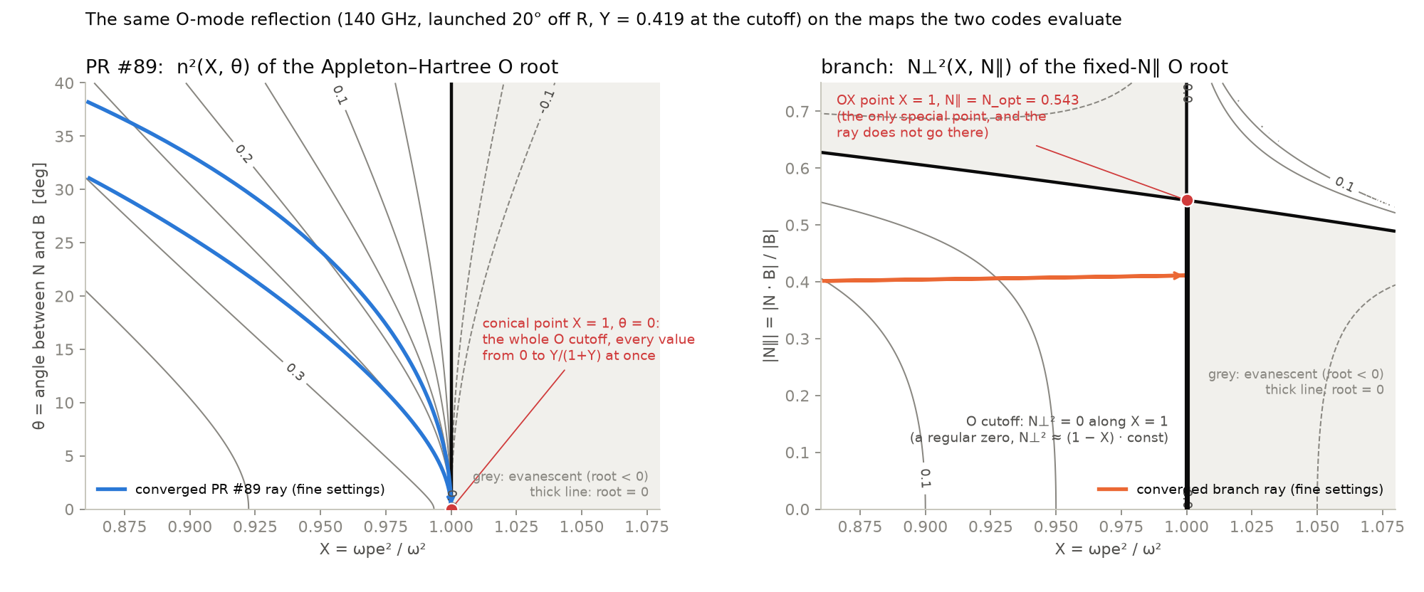
The reflection of section 1 drawn on the two maps the codes evaluate, both at the Y of the turning point. Left: the Appleton–Hartree O root over (X, θ); every contour between 0 and Y/(1 + Y) ends at the conical point, and the converged PR #89 ray runs into that point to turn around. There the trial points of a Runge–Kutta step land on different contours, H differs between them by order one whatever the step size, and the error estimate of the step, which assumes a smooth right-hand side, is meaningless. Right: the branch's root over (X, N∥); the contours are a regular family, the zero line is X = 1 up to N_opt, and the ray turns at a regular point of it. The only special point of this map is the OX point, which the ray does not visit.
2.2 Hamiltonian time, because the group velocity vanishes at the cutoff
On the cutoff segment$\partial H/\partial\mathbf N=0$ for every regular form of $H$ , because $H$ carries the factor $N_\perp^2$ there: the O mode stops at its cutoff, at oblique incidence too. PR #89 divides the right-hand side by $\lvert\partial H/\partial\mathbf N\rvert$ to integrate in the arc length, which is 0/0 at the reflection: the unit tangent flips by 180° and the path has a cusp. In Hamiltonian time the same point is regular, with $N_\perp\simeq-\kappa t$ and $x_c-x\simeq\kappa t^2$ in a slab, so the branch integrates
with the state$(\mathbf r,\mathbf N,\tau,s)$ . The arc length is integrated alongside, so that it stays the coordinate of the output profiles and of
max_arc_length, but it is left out of the error norm: it is an output, its error does not feed back into the ray, and the step sequence is that of the state without it. The controller uses its increment to expressmax_step_sizein metres and to reject a step longer than 1.5 ×max_step_size. The same Hamiltonian integrated in the arc length, everything else equal, needs 2–3 × the steps at every reflection and loses 3 of 10 OX launches to NaN: the cusp is physics, not a property of the formula.2.3 The step error as a frequency mismatch
since$\mathbf N=c\mathbf k/\omega$ . This is the relative change of frequency that would put the wave back on the dispersion surface. To first order it is the same for $H$ and for $f\cdot H$ with any smooth non-zero $f$ , so it measures the ray and not the form of $H$ ; it stays finite at the reflection, where $\partial H/\partial\mathbf N$ vanishes but $\partial H/\partial\omega$ does not; and it is what the physicist would check. It replaces $\Delta H/(2\lvert\mathbf N\rvert)$ in the same place of the same controller, weighted by $\partial H/\partial\omega$ comes out of the same reverse pass as $\partial H/\partial\mathbf N$ . The old measure is the change of $\lvert\mathbf N\rvert$ only when $n^2$ does not depend on $\mathbf N$ , which is not the case for the angle form, and it diverges at $\lvert\mathbf N\rvert\to0$ , where an O-mode ray at normal incidence turns.
dispersion_error_weight= 30 against the relative tolerance, at the same cost:3. The other rays
The same tokamak at 140, 42 and 56 GHz, so that Y is below 1, above 1 or crosses 1 along the ray; O and X mode; a low density that lets the ray through and a high density that reflects it; launched at 0°, 20° and 45°. The three O-mode reflections at 20° are the ones that go wrong on PR #89; the figure shows them, the tables below give all 36 rays and the OX scan.
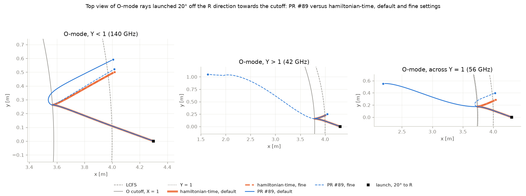
O-mode rays at 20° reaching their cutoff, top view. Solid: shipped settings, dashed: fine settings. At 42 GHz (Y > 1) the fine run of PR #89 goes through the cutoff and ends on the high-field side; at 56 GHz (Y = 1 inside the plasma) its shipped run runs out of steps beyond the cutoff. On the branch the four runs of each case lie on top of each other.
Mode scan, 36 rays: end-point distance between the shipped and the fine run
✅ both runs finish on the same side, end points within 1 mm, |δω/ω| below 10⁻³ along the shipped run.⚠️ finished, but off. ❌ NaN or out of steps. The X-mode ray at 42 GHz and 45° on the branch is the fold of section 4; the X-mode rays from the high-field side at 56 GHz cross the upper-hybrid resonance, where neither code stops.
OX reflection scan: O mode started 1 or 3 mm outside its cutoff with N∥ near the OX optimum, traced out, reversed and traced back through the reflection
The evanescent layer between the O cutoff and the Z-mode cutoff has the thickness$\Delta X=Y,(1-f^2)$ for $N_\parallel=fN_{\rm opt}$ , listed in mm. "Passed the cutoff" means X_max > 1.005: the ray continued on the X-mode sheet. The distance is to the same code's converged run without H term; on PR #89 that reference itself passes the cutoff in three launches.
4. What remains
RayState,TraceBuffers,BeamProfileandTracerSettingskeep their fields and their meaning.max_arc_lengthis a second termination condition on the integrated arc length, root-found like the exit from the plasma, so the ray ends at that length itself andTraceResult.incompleteis set as before.max_step_sizeacts through |∂H/∂N| at the start of the step and the rejection above 1.5 × its value.5. In the code
physics/dispersion.py(refractive_index_perp_squared_cold),physics/hamiltonian.py(the new H),tracer/solver.py(Hamiltonian time, frequency-mismatch controller, arc-length event); docstrings intypes.pyandtracer/buffers.py, one line inapi.py. The ODE state is (r, N, τ, s): eight components instead of seven, the eighth outside the error norm and at no extra cost, since ∂H/∂N is computed anyway. One commit on top ofmain.theory/ray-tracing.md(Hamiltonian time, the fixed-N∥ root and why not the angle form, the frequency mismatch),limitations.md(OX conversion and gap, the fold, the upper-hybrid resonance),tuning.md(whatdispersion_error_weightmeasures, the reflection step), and the map figure of section 2 asdocs/assets/cutoff_maps.png. The sign statement for the Appleton–Hartree formula on the theory page is corrected: theruff,mypyandpytestpass (387 tests passed; the plot tests need pyvista and were not run). New tests: the root lies on the Appleton–Hartree sheet of its mode for Y = 0.3, 0.95, 1, 1.05, 2; the vacuum limit and its derivative; the linear zero of the O root at its reflection point; an API-level reflection test for O and X at 0° and 25° (shipped and converged end points within 1 mm, no crossing of the cutoff, R Nφ conserved).jax.gradis 2.356 m/rad against 2.350 by central differences. For the total arc length the converged value is 0.848 m/rad (fine settings, AD and differences agree to 0.3 %); with the shipped settings AD gives 0.816 and central differences scatter between 0.5 and 0.87 with their step, because the one step that contains the cusp integrates |∂H/∂N| across its kink with an error of a few tens of micrometres that moves with the launch angle. On PR Control steps on the change of H instead of relaxing back to H = 0 #89 the end-point derivative is 4·10⁶ by AD and −117 by differences: at the conical point it does not exist.